Diffusion models for ultrasound image generation

In this notebook, we will look at one of the current state-of-the-art deep generative models: diffusion models. These models have shown great promise in generating high-quality images and have been applied to various tasks, including ultrasound synthesis, inpainting, but also denoising / dehazing of ultrasound images. zea.Models supports some pretrained diffusion models, ready to perform prior and posterior sampling. We’ll start, as always with setting the Keras backend.

   

%%capture
%pip install zea

import os

os.environ["KERAS_BACKEND"] = "jax"
os.environ["TF_CPP_MIN_LOG_LEVEL"] = "2"

import keras
from zea import log, init_device
from zea.models.diffusion import DiffusionModel
from zea.ops import Pipeline, ScanConvert
from zea.data import Dataset
from zea.visualize import plot_image_grid, set_mpl_style
from zea.agent.selection import EquispacedLines
from zea.utils import translate

zea: Using backend 'jax'

We’ll use the following parameters for this experiment.

n_unconditional_samples = 16
n_unconditional_steps = 90
n_conditional_samples = 4
n_conditional_steps = 200

We will work with the GPU if available, and initialize using init_device to pick the best available device. Also, (optionally), we will set the matplotlib style for plotting.

init_device(verbose=False)
set_mpl_style()

Unconditional generation

Let’s choose a pretrained diffusion model (on EchoNet Dynamic dataset) and generate some ultrasound images. Using presets.keys() we can see the available models. One could also point to a custom model by passing a local path to the model checkpoint directory.

presets = list(DiffusionModel.presets.keys())
log.info(f"Available built-in zea presets for DiffusionModel: {presets}")

model = DiffusionModel.from_preset("diffusion-echonet-dynamic")  # or use a local path to your model

# Prior sampling
prior_samples = model.sample(
    n_samples=n_unconditional_samples, n_steps=n_unconditional_steps, verbose=True
)

zea: Available built-in zea presets for DiffusionModel: ['diffusion-echonet-dynamic']
90/90 ━━━━━━━━━━━━━━━━━━━━ 23s 88ms/step

Postprocessing

Now we have generated the images, we want to postprocess them a bit (in this case, scanconvert to Cartesian grid). We can use the zea.Pipeline class to easily create a processing pipeline.

pipeline = Pipeline([ScanConvert(order=2, jit_compile=False)])
parameters = {
    "theta_range": [-0.78, 0.78],  # [-45, 45] in radians
    "rho_range": [0, 1],
}
processed_batch = keras.ops.squeeze(prior_samples, axis=-1)

parameters = pipeline.prepare_parameters(**parameters)
processed_batch = pipeline(data=processed_batch, **parameters)["data"]

zea: WARNING GPU support for order > 1 is not available. Disabling jit for ScanConvert.

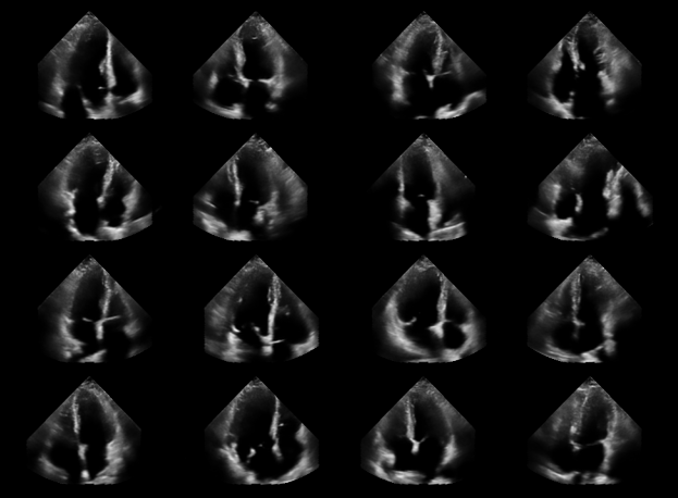
fig, _ = plot_image_grid(
    processed_batch,
    vmin=-1,
    vmax=1,
)

Dataset loading

Generating unconditional ultrasound images is nice, but we can also perform a task with these generative diffusion models. For example, we can inpaint missing regions that were not acquired during the ultrasound scan. We can use the posterior_sample() method to generate samples conditioned on a measurement, given some measurement model.

First we need some actual ultrasound data to condition on. We can use the zea.Dataset class to load a dataset from Huggingface, or from a local path.

dataset = Dataset("hf://zeahub/camus-sample/val", key="image")

data = dataset[0]["data"]["image"]

img_shape = model.input_shape[:2]

data = keras.ops.expand_dims(data, axis=-1)
data = keras.ops.image.resize(data, img_shape)
dynamic_range = (-40, 0)
data = keras.ops.clip(data, dynamic_range[0], dynamic_range[1])
data = translate(data, dynamic_range, (-1, 1))

zea: Using pregenerated dataset info file: /home/devcontainer15/.cache/zea/huggingface/datasets/datasets--zeahub--camus-sample/snapshots/617cf91a1267b5ffbcfafe9bebf0813c7cee8493/val/dataset_info.yaml ...
zea: ...for reading file paths in /home/devcontainer15/.cache/zea/huggingface/datasets/datasets--zeahub--camus-sample/snapshots/617cf91a1267b5ffbcfafe9bebf0813c7cee8493/val
zea: Dataset was validated on July 17, 2025
zea: Remove /home/devcontainer15/.cache/zea/huggingface/datasets/datasets--zeahub--camus-sample/snapshots/617cf91a1267b5ffbcfafe9bebf0813c7cee8493/val/validated.flag if you want to redo validation.

We can then create the measurement, by subsampling the original data using a mask.

line_thickness = 2
factor = 2
agent = EquispacedLines(
    n_actions=img_shape[1] // line_thickness // factor,
    n_possible_actions=img_shape[1] // line_thickness,
    img_width=img_shape[1],
    img_height=img_shape[0],
)

_, mask = agent.sample(batch_size=len(data))
mask = keras.ops.expand_dims(mask, axis=-1)

measurements = keras.ops.where(mask, data, -1.0)

Posterior sampling (conditional generation)

Finally, we can use the posterior_sample() method to generate samples conditioned on the measurement. The posterior_sample() method takes a measurement and a measurement model as input, and returns a posterior sample. We can draw multiple samples and visualize the posterior variance as a proxy to see how uncertain the model is about the missing regions.

## Posterior sampling
posterior_samples = model.posterior_sample(
    measurements=measurements,
    mask=mask,
    n_samples=n_conditional_samples,
    n_steps=n_conditional_steps,
    omega=30.0,
    verbose=True,
)
posterior_variance = keras.ops.var(posterior_samples, axis=1)
posterior_samples = posterior_samples[:, 0]  # Get first sample only
# scale posterior variance to [-1, 1] range so it can be visualized
posterior_variance = translate(
    posterior_variance,
    (0, keras.ops.max(posterior_variance)),
    (-1, 1),
)

## Post processing (ScanConvert)
concatenated = [prior_samples, data, measurements, posterior_samples, posterior_variance]
# limit number of samples for visualization
concatenated = [sample[:n_conditional_samples] for sample in concatenated]
concatenated = keras.ops.concatenate(concatenated, axis=0)
concatenated = keras.ops.squeeze(concatenated, axis=-1)

processed_batch = pipeline(data=concatenated, **parameters)["data"]

200/200 ━━━━━━━━━━━━━━━━━━━━ 41s 117ms/step - error: 20046.6328

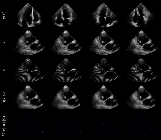
And now let’s visualize the results! We will show some prior samples, the original target images (CAMUS dataset), the measurement, and the posterior samples. We can also visualize the posterior variance as a proxy for uncertainty.

In short:

• Prior samples: x ~ p(x), sampled from the diffusion model trained on the EchoNet Dynamic dataset

• Original image: x, from the CAMUS dataset

• Measurement: y, a masked version of x

• Posterior samples: x ~ p(x|y), sampled from the diffusion model conditioned on the measurement y

• Posterior variance: Var[p(x|y)], visualized as a heatmap to show uncertainty in the posterior samples

n_rows = 5  # prior, batch, measurements, posterior, posterior_variance
imgs_per_row = n_conditional_samples

cmaps = ["gray"] * ((n_rows - 1) * imgs_per_row) + ["inferno"] * imgs_per_row

## Plotting
fig, _ = plot_image_grid(
    processed_batch,
    vmin=-1,
    vmax=1,
    remove_axis=False,
    ncols=imgs_per_row,
    cmap=cmaps,
)

titles = ["p(x)", "x", "y", "p(x|y)", "Var[p(x|y)]"]

for i, title in enumerate(titles):
    fig.axes[i * imgs_per_row].set_ylabel(title)