Working with the zea data format

In this tutorial notebook we will show how to load a zea data file and how to access the data stored in it. There are three common ways to load a zea data file:

1. Loading data from single file with zea.File

2. Loading data from a group of files with zea.Dataset

3. Loading data in batches with dataloading utilities with zea.backend.tensorflow.make_dataloader

   

%%capture
%pip install zea

config_picmus_iq = "hf://zeahub/configs/config_picmus_iq.yaml"

import os

os.environ["KERAS_BACKEND"] = "jax"
os.environ["ZEA_DISABLE_CACHE"] = "1"
os.environ["TF_CPP_MIN_LOG_LEVEL"] = "3"

import matplotlib.pyplot as plt

import zea
from zea import init_device, load_file
from zea.visualize import set_mpl_style
from zea.backend.tensorflow import make_dataloader

zea: Using backend 'jax'

We will work with the GPU if available, and initialize using init_device to pick the best available device. Also, (optionally), we will set the matplotlib style for plotting.

init_device(verbose=False)
set_mpl_style()

Loading a file with zea.File

The zea data format works with HDF5 files. We can open a zea data file using the h5py package and have a look at the contents using the zea.File.summary() function. You can see that every dataset element contains a corresponding description and unit. Note that we now pass a url to a Hugging Face dataset, but you can also use a local file path to a zea data file. Here we will use an example from the PICMUS dataset, converted to zea format and hosted on the Hugging Face Hub.

Tip: You can also use the HDFView tool to view the contents of the zea data file without having to run any code. Or if you use VS Code, you can install the HDF5 extension to view the contents of the file.

You can extract data and acquisition parameters (which are stored together with the data in the zea data file) as follows:

file_path = "hf://zeahub/picmus/database/experiments/contrast_speckle/contrast_speckle_expe_dataset_iq/contrast_speckle_expe_dataset_iq.hdf5"

with zea.File(file_path, mode="r") as file:
    file.summary()

    data = file.load_data("raw_data", indices=[0])
    scan = file.scan()
    probe = file.probe()

contrast_speckle_expe_dataset_iq.hdf5/
    ├── description: PICMUS dataset converted to USBMD format
    ├── probe: verasonics_l11_4v
    ├── data/
    │   ├── description: This group contains the data.
    │   └── raw_data/
    │       ├── /data/raw_data (shape=(1, 75, 832, 128, 2))
    │       │   ├── description: The raw_data of shape (n_frames, n_tx, n_el, n_ax, n_ch).
    │       │   ├── unit: unitless
    └── scan/
        ├── description: This group contains the scan parameters.
        ├── azimuth_angles/
        │   ├── /scan/azimuth_angles (shape=(75))
        │   │   ├── description: The azimuthal angles of the transmit beams in radians of shape (n_tx,).
        │   │   ├── unit: rad
        ├── center_frequency/
        │   ├── /scan/center_frequency (shape=())
        │   │   ├── description: The center frequency in Hz.
        │   │   ├── unit: Hz
        ├── focus_distances/
        │   ├── /scan/focus_distances (shape=(75))
        │   │   ├── description: The transmit focus distances in meters of shape (n_tx,). For planewaves this is set to Inf.
        │   │   ├── unit: m
        ├── initial_times/
        │   ├── /scan/initial_times (shape=(75))
        │   │   ├── description: The times when the A/D converter starts sampling in seconds of shape (n_tx,). This is the time between the first element firing and the first recorded sample.
        │   │   ├── unit: s
        ├── n_ax/
        │   ├── /scan/n_ax (shape=())
        │   │   ├── description: The number of axial samples.
        │   │   ├── unit: unitless
        ├── n_el/
        │   ├── /scan/n_el (shape=())
        │   │   ├── description: The number of elements in the probe.
        │   │   ├── unit: unitless
        ├── n_frames/
        │   ├── /scan/n_frames (shape=())
        │   │   ├── description: The number of frames.
        │   │   ├── unit: unitless
        ├── n_tx/
        │   ├── /scan/n_tx (shape=())
        │   │   ├── description: The number of transmits per frame.
        │   │   ├── unit: unitless
        ├── polar_angles/
        │   ├── /scan/polar_angles (shape=(75))
        │   │   ├── description: The polar angles of the transmit beams in radians of shape (n_tx,).
        │   │   ├── unit: rad
        ├── probe_geometry/
        │   ├── /scan/probe_geometry (shape=(128, 3))
        │   │   ├── description: The probe geometry of shape (n_el, 3).
        │   │   ├── unit: m
        ├── sampling_frequency/
        │   ├── /scan/sampling_frequency (shape=())
        │   │   ├── description: The sampling frequency in Hz.
        │   │   ├── unit: Hz
        ├── sound_speed/
        │   ├── /scan/sound_speed (shape=())
        │   │   ├── description: The speed of sound in m/s
        │   │   ├── unit: m/s
        ├── t0_delays/
        │   ├── /scan/t0_delays (shape=(75, 128))
        │   │   ├── description: The t0_delays of shape (n_tx, n_el).
        │   │   ├── unit: s
        └── tx_apodizations/
            ├── /scan/tx_apodizations (shape=(75, 128))
            │   ├── description: The transmit delays for each element defining the wavefront in seconds of shape (n_tx, n_elem). This is the time at which each element fires shifted such that the first element fires at t=0.
            │   ├── unit: unitless

You can also do this exact thing in one go using zea.load_file which will directly return you the data and parameter objects.

data, scan, probe = load_file(file_path, "raw_data", indices=[[0], slice(0, 3)])

print("Raw data shape:", data.shape)
print(scan)
print(probe)

Raw data shape: (1, 3, 832, 128, 2)
<zea.scan.Scan object at 0x7f92a0101780>
<zea.probes.Verasonics_l11_4v object at 0x7f9183bf92a0>

Loading data with zea.Dataset

We can also load and manage a group of files (i.e. a dataset) using the zea.Dataset class. Instead of a path to a single file, we can pass a list of file paths or a directory containing multiple zea data files. The zea.Dataset class will automatically load the files and allow you to access the data in a similar way as with zea.File.

dataset_path = "hf://zeahub/picmus/database/experiments"

dataset = zea.Dataset(dataset_path, key="raw_data")

print(dataset)

for file in dataset:
    print(file)

dataset.close()

zea: Searching /tmp/zea_cache_7c7p3ydn/huggingface/datasets/datasets--zeahub--picmus/snapshots/79a57eaa7e4e284cf6bef10df33cc0bdce400190/database/experiments for ['.hdf5', '.h5'] files...
zea: Getting number of frames in each hdf5 file...

Getting number of frames in each hdf5 file: 100%|██████████| 4/4 [00:00<00:00, 1158.97it/s]

zea: Found 4 image files in /tmp/zea_cache_7c7p3ydn/huggingface/datasets/datasets--zeahub--picmus/snapshots/79a57eaa7e4e284cf6bef10df33cc0bdce400190/database/experiments
zea: Writing dataset info to /tmp/zea_cache_7c7p3ydn/huggingface/datasets/datasets--zeahub--picmus/snapshots/79a57eaa7e4e284cf6bef10df33cc0bdce400190/database/experiments/dataset_info.yaml

Checking dataset files on validity (zea format): 100%|██████████| 4/4 [00:00<00:00, 88.40it/s]

zea: Dataset validated. Check /tmp/zea_cache_7c7p3ydn/huggingface/datasets/datasets--zeahub--picmus/snapshots/79a57eaa7e4e284cf6bef10df33cc0bdce400190/database/experiments/validated.flag for details.
Dataset with 4 files (key='raw_data')
zea HDF5 File: 'contrast_speckle_expe_dataset_rf.hdf5' (mode=r)
zea HDF5 File: 'contrast_speckle_expe_dataset_iq.hdf5' (mode=r)
zea HDF5 File: 'resolution_distorsion_expe_dataset_iq.hdf5' (mode=r)
zea HDF5 File: 'resolution_distorsion_expe_dataset_rf.hdf5' (mode=r)
zea: Closed all cached file handles.

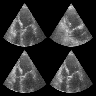
Loading data with make_dataloader

In machine and deep learning workflows, we often want more features like batching, shuffling, and parallel data loading. The zea.backend.tensorflow.make_dataloader function provides a convenient way to create a TensorFlow data loader from a zea dataset. This does require a working TensorFlow installation, but does work in combination with any other backend as well. This dataloader is particularly useful for training models. It is important that there is some consistency in the dataset, which is not the case for PICMUS. Therefore in this example we will use a small part of the CAMUS dataset.

dataset_path = "hf://zeahub/camus-sample/val"
dataloader = make_dataloader(
    dataset_path,
    key="data/image_sc",
    batch_size=4,
    shuffle=True,
    clip_image_range=[-60, 0],
    image_range=[-60, 0],
    normalization_range=[0, 1],
    image_size=(256, 256),
    resize_type="resize",  # or "center_crop or "random_crop"
    seed=4,
)

for batch in dataloader:
    print("Batch shape:", batch.shape)
    break  # Just show the first batch

fig, _ = zea.visualize.plot_image_grid(batch)

zea: Searching /tmp/zea_cache_7c7p3ydn/huggingface/datasets/datasets--zeahub--camus-sample/snapshots/617cf91a1267b5ffbcfafe9bebf0813c7cee8493/val for ['.hdf5', '.h5'] files...
zea: Getting number of frames in each hdf5 file...

Getting number of frames in each hdf5 file: 100%|██████████| 2/2 [00:00<00:00, 818.32it/s]

zea: Found 2 image files in /tmp/zea_cache_7c7p3ydn/huggingface/datasets/datasets--zeahub--camus-sample/snapshots/617cf91a1267b5ffbcfafe9bebf0813c7cee8493/val
zea: Writing dataset info to /tmp/zea_cache_7c7p3ydn/huggingface/datasets/datasets--zeahub--camus-sample/snapshots/617cf91a1267b5ffbcfafe9bebf0813c7cee8493/val/dataset_info.yaml

Checking dataset files on validity (zea format): 100%|██████████| 2/2 [00:00<00:00, 183.30it/s]

zea: Dataset validated. Check /tmp/zea_cache_7c7p3ydn/huggingface/datasets/datasets--zeahub--camus-sample/snapshots/617cf91a1267b5ffbcfafe9bebf0813c7cee8493/val/validated.flag for details.
zea: WARNING H5Generator: Not all files have the same shape. This can lead to issues when resizing images later....
zea: H5Generator: Shuffled data.

zea: H5Generator: Shuffled data.
Batch shape: (4, 256, 256, 1)

Processing an example

We will now use one of the zea data files to demonstrate how to process it. A full example can be found in the zea_pipeline_example notebook. Here we will just show a simple example for completeness. We will start by loading a config file, that contains all the required information to initiate a processing pipeline.

config = zea.Config.from_path(config_picmus_iq)

Now we can load the zea data file, extract data and parameters, and then process the data using the pipeline defined by the config file.

with zea.File(config.data.dataset_folder + "/" + config.data.file_path, mode="r") as file:
    # we use config here to overwrite some of the scan parameters
    scan = file.scan(**config.scan)
    data = file.load_data(config.data.dtype)

pipeline = zea.Pipeline.from_config(config.pipeline)
parameters = pipeline.prepare_parameters(probe=probe, scan=scan)

images = pipeline(data=data, **parameters)["data"]

zea: Caching is globally disabled for compute_pfield.
zea: Computing pressure field for all transmits
75/75 ━━━━━━━━━━━━━━━━━━━━ 15s 105ms/transmits

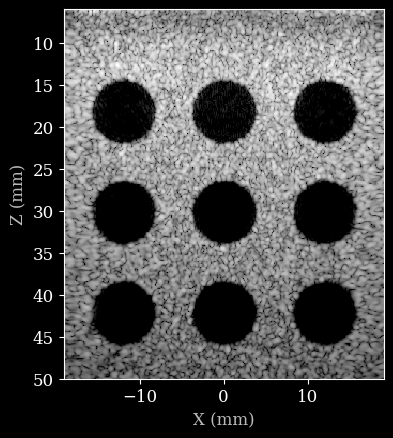
Finally we can plot the result.

image = zea.display.to_8bit(images[0], dynamic_range=(-50, 0))
plt.figure()
# Convert xlims and zlims from meters to millimeters for display
xlims_mm = [v * 1e3 for v in scan.xlims]
zlims_mm = [v * 1e3 for v in scan.zlims]
plt.imshow(image, cmap="gray", extent=[xlims_mm[0], xlims_mm[1], zlims_mm[1], zlims_mm[0]])
plt.xlabel("X (mm)")
plt.ylabel("Z (mm)")

Text(0, 0.5, 'Z (mm)')